
System Design 101: How to Scale Databases with Partitioning
Scale your database beyond a single server. Master the three core partitioning strategies, Range, Hash, and Directory-Based Sharding, and learn how to prevent Hotspots and handle Resharding.

Every computer system eventually faces a physical limit.
No matter how much money you spend, you cannot buy a processor with infinite speed or a hard drive with infinite capacity.
There is a finite limit to how many requests a single machine can handle before it slows down, queues requests, or crashes entirely.
When a database reaches this limit, vertical scaling (buying a bigger computer) is no longer an option.
You must switch to horizontal scaling. This means adding more computers to the pool and splitting your data across them.
In system design, we call this Partitioning or Sharding.
However, splitting the data is the easy part. The difficult part is retrieval.
When you have a single server, the application always knows where to look. But when you have ten servers, the application faces a critical question for every single query: Which of these ten servers holds the specific record I need?
If the application does not know the answer, it has to ask every single server. This is inefficient and slow.
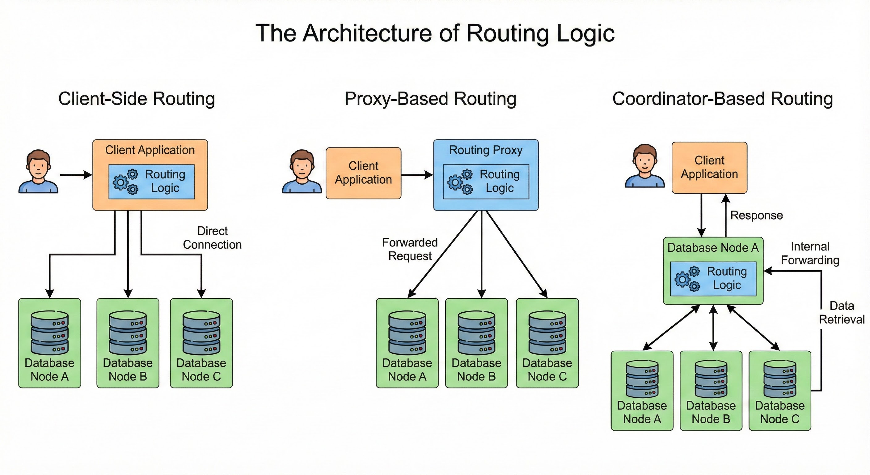
To build a scalable system, the application needs a precise way to determine the location of data before it even opens a connection.
This set of rules is called Routing Logic.
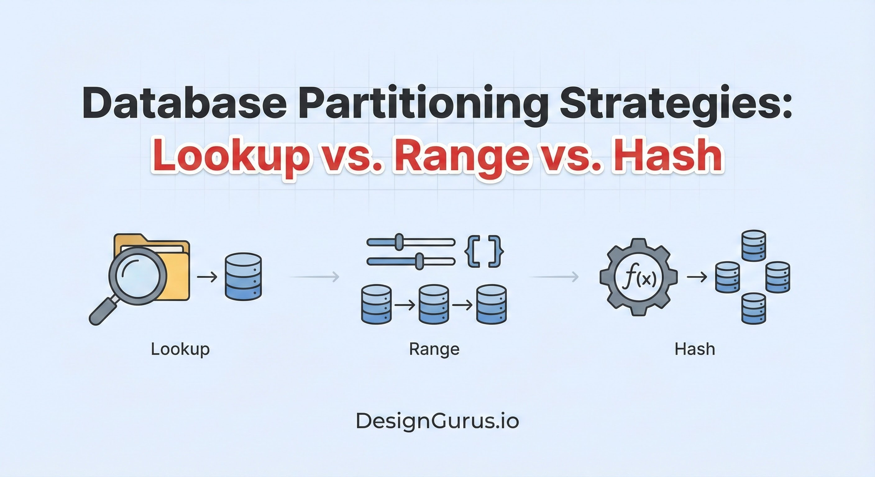
In this guide, we will explore the internal mechanics of this logic. We will look at how applications use Range Partitioning, Hash Partitioning, and Directory-Based Partitioning to solve the routing problem.
The Core Concept: The Partition Key
Before we analyze the strategies, we must define the input for our routing logic. This is the Partition Key.
When you write a row of data to a database, you must choose one specific column or attribute to act as the primary identifier for routing. This is usually a unique ID, such as a User ID, a Transaction ID, or a Timestamp.
The routing logic is a function. It takes this Partition Key as an input and outputs a server address.
Server Address = Function(Partition Key)
The goal of system design is to choose a function that distributes data evenly across all your servers.
If the function is poorly designed, it will send all the data to one server while the others sit empty. We call this uneven distribution a Hotspot or Data Skew.
Strategy 1: Range Partitioning
Range Partitioning is the most intuitive strategy to understand. It assigns data to servers based on continuous sequences of values.
You define strict boundaries (ranges), and the routing logic simply checks which range the Partition Key falls into.
How the Routing Logic Works
The application or the database proxy holds a configuration map in memory. This map defines the boundaries for every connected server.
Consider a system that stores Customer Orders. We use the Order_ID as the Partition Key. The routing logic might look like this:
Input: The application initiates a query for
Order_ID: 15,000.Logic Check: The router checks the configured ranges.
Node A: Handles IDs 1 to 10,000.
Node B: Handles IDs 10,001 to 20,000.
Node C: Handles IDs 20,001 to 30,000.
Routing: The router determines that 15,000 is greater than 10,001 but less than 20,000.
Output: The request is sent specifically to Node B.
Why Choose Range Partitioning?
The primary strength of this strategy is the efficiency of Range Scans.
A range scan is a query that requests a group of related items.
For example, “Get all orders between ID 100 and ID 200.” Because of the routing logic, the system knows that IDs 100 through 200 are all stored on the same server (Node A).
The application sends a single request to Node A, retrieves all the records, and returns them.
If the data were scattered randomly across all nodes, the application would have to connect to Node A, Node B, and Node C, execute the query on all of them, and then combine the results.
Range partitioning avoids this overhead.
The Technical Limitation: Hotspots
Range partitioning is very susceptible to hotspots, particularly with time-series data.
If you partition by Creation_Date, you might assign “January Data” to Node A and “February Data” to Node B.
During the month of February, 100% of the write traffic and most of the read traffic will hit Node B.
Node A will be effectively offline because no one is reading old data.
This creates an imbalance where one server is overloaded and the others are underutilized, limiting the total capacity of the system to the capacity of a single node.
Strategy 2: Algorithmic Partitioning (Hash)
To solve the hotspot problem, we need to ensure that data is spread uniformly across the cluster.
We want sequential data (like Order 1, Order 2, Order 3) to be placed on different servers.
To achieve this, we use Hash Partitioning. This is an algorithmic approach that uses mathematics rather than a static configuration map.
How the Routing Logic Works
This strategy relies on a hash function and the modulo operator.
A hash function takes an arbitrary input (the Partition Key) and converts it into a fixed integer (a hash value). This integer looks random but is deterministic. The same input will always produce the same integer.
The modulo operator (represented as %) calculates the remainder of a division operation.
The routing formula is generally:
Shard_Index = Hash(Key) % Number_of_Servers
Let us trace the execution flow for a system with 3 Servers (Server 0, Server 1, Server 2).
Request 1: Write data for User_ID: 100.
The system hashes “100”. Result:
350.The system calculates
350 % 3.350 divided by 3 is 116 with a remainder of 2.
Destination: Server 2.
Request 2: Write data for User_ID: 101.
The system hashes “101”. Result:
802.The system calculates
802 % 3.802 divided by 3 is 267 with a remainder of 1.
Destination: Server 1.
Even though the User IDs (100 and 101) are sequential, the math forces them onto different servers.
Why Choose Hash Partitioning?
The benefit is Uniform Distribution.
The randomized nature of the hash function ensures that data is evenly scattered.
