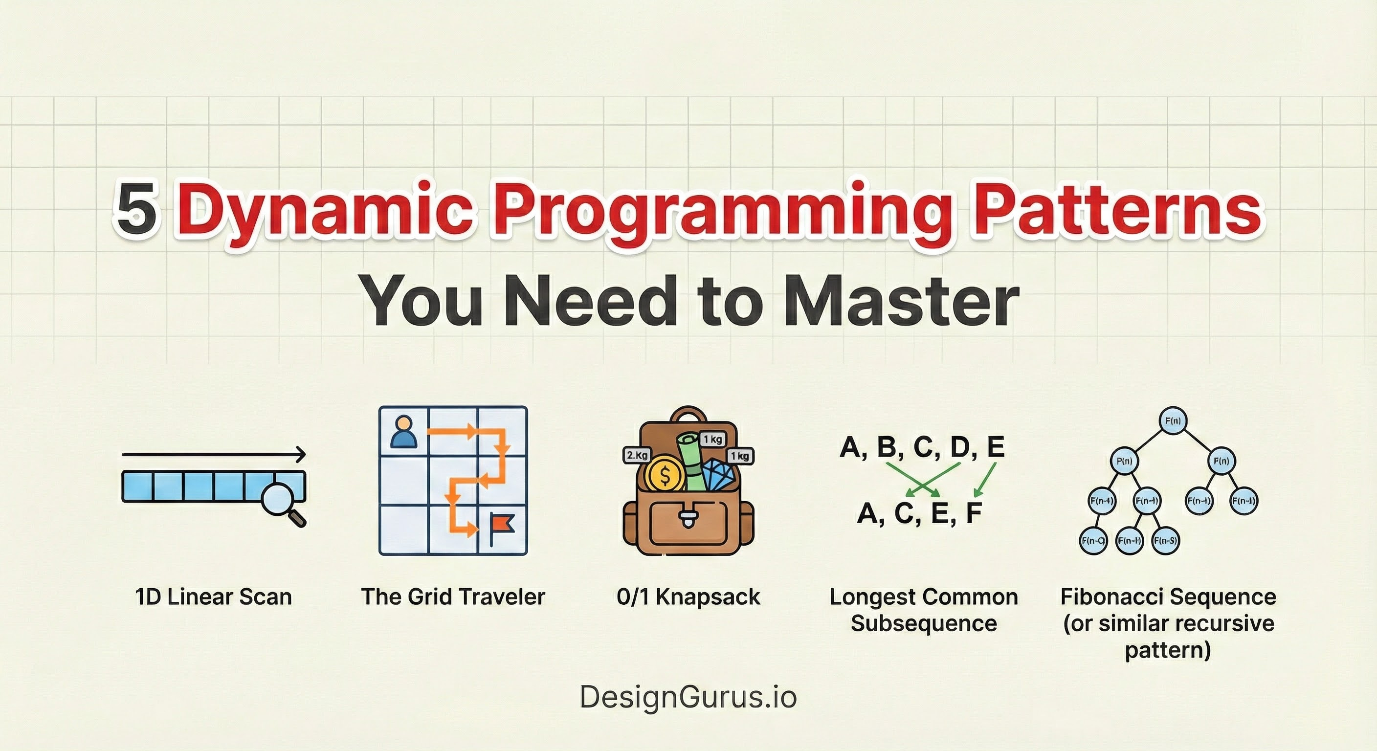
Dynamic Programming Decoded: 6 Patterns to Solve Any Interview Problem

Stop fearing Dynamic Programming. Master the difference between Memoization and Tabulation, and learn 6 essential patterns, including the Knapsack Problem, Grid Traveler, and LCS.

Dynamic Programming sounds scary, but it is actually simple. It is just a fancy way of saying "remember what you learned."

Many code solutions are slow because they solve the same small problem over and over again.

This wastes time.

The fix is to save your answers so you never do the same work twice.

In this guide, we will show you the exact dynamic programming patterns you need to turn slow code into instant solutions. It is time to work smarter.

What is Dynamic Programming?

Dynamic Programming is a method for solving complex problems by breaking them down into simpler subproblems. It solves each subproblem just once and stores the result.

When you see the same subproblem occur again, you do not recalculate it. You simply look up the stored result.

There are two main properties a problem must have to be solved with DP:

1. Overlapping Subproblems: The code asks for the same result multiple times during execution.

2. Optimal Substructure: The optimal solution to the big problem can be constructed from the optimal solutions of the subproblems.

If you have these two things, you can use DP.

The Two Approaches: Top-Down vs. Bottom-Up

Before we look at patterns, you need to know the two ways to implement DP.

Memoization (Top-Down)

This is the easier approach if you are comfortable with recursion. You start with the large problem and break it down.

Imagine a recursive function. Normally, it calls itself blindly.

In Memoization, you add a check at the start of the function. You ask, “Have I solved this specific input before?”

If yes, you return the stored answer from a hash map or array.

If no, you do the calculation, store the answer, and then return it.

We call this “Top-Down” because you start at the top (the final goal) and dig down to the base cases.

Tabulation (Bottom-Up)

This approach avoids recursion entirely. It uses loops.

You start with the smallest possible subproblem (the base case).

You fill up a table (usually an array or a matrix) with these small answers.

Then, you use those answers to calculate slightly larger problems. You keep building up until you reach the final answer.

We call this “Bottom-Up” because you start at the bottom (the base cases) and build up to the goal.

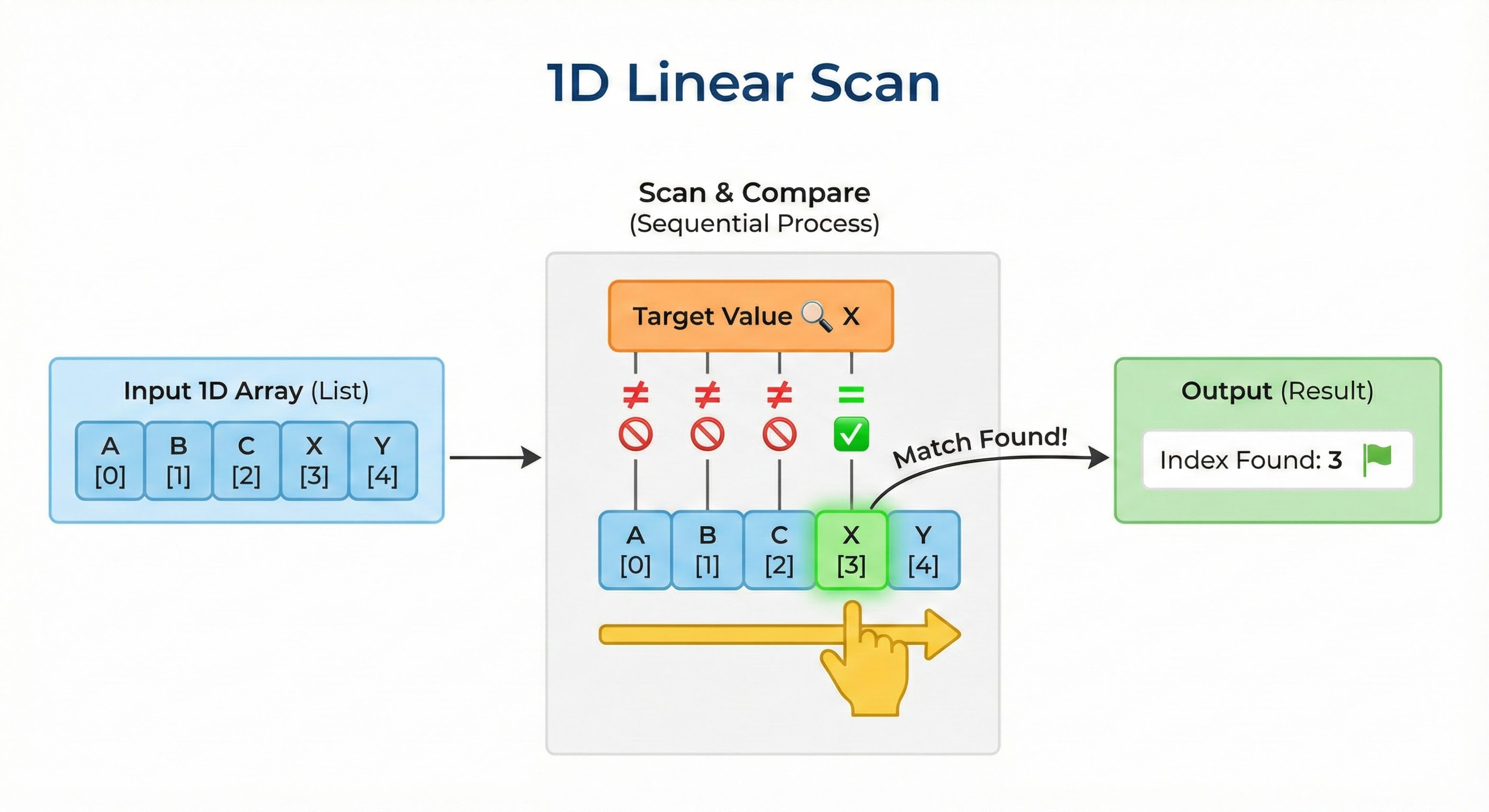
Pattern 1: The 1D Linear Scan

This is the most basic pattern. It usually involves an array or a sequence of numbers.

The Logic: The value at the current index i depends only on the values at previous indices, usually i-1 and i-2.

How to Spot It: The problem asks for the total number of ways to reach a target or the max/min value in a sequence. You can only move forward.

The State Transition: To solve for index i, you look at where you could have come from. If you can move 1 step or 2 steps at a time, the equation looks like this: dp[i] = dp[i-1] + dp[i-2]

Walkthrough

1. Create an array dp of size N.

2. Set the base cases. Usually dp[0] and dp[1] are known values.

3. Loop from 2 up to N.

4. Apply the formula inside the loop.

5. The answer is in dp[N].

This pattern teaches you that the “future” result is just a combination of “past” results.

Pattern 2: The Grid Traveler

Now we add a dimension.

Instead of a line, you are on a 2D matrix.

The Logic: You are usually at the top-left cell (0, 0) and need to reach the bottom-right cell (m, n). You can typically move only down or right.

How to Spot It: The problem involves a board, a grid, or a matrix. It asks for the number of distinct paths or the minimum/maximum cost to traverse the grid.

The State Transition: Think about a random cell in the middle of the grid at [r][c]. How did you get there? Since you can only move down or right, you must have arrived from the cell directly above it or the cell directly to the left of it.

Therefore, the value at the current cell is a function of the cell above and the cell to the left. dp[r][c] = dp[r-1][c] + dp[r][c-1]

Walkthrough

1. Create a 2D matrix of the same size.

2. Initialize the first row and first column. There is usually only one way to reach any cell in the first row (move right) or first column (move down).

3. Iterate through the rest of the grid with a nested loop.

4. Apply the logic: Current Cell = Top Cell + Left Cell.

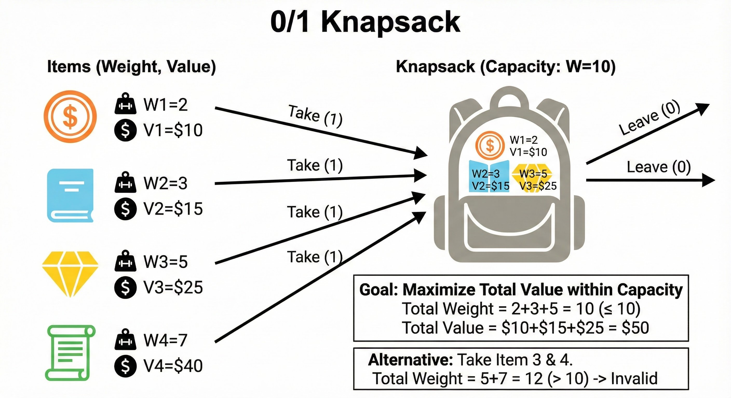
Pattern 3: The 0/1 Knapsack

This is perhaps the most famous pattern in optimization.

The Logic: You have a set of items. Each item has a value and a weight. You also have a maximum capacity. For every item, you have a binary choice:

1. Include the item in your set.

2. Exclude the item from your set.

How to Spot It: You need to maximize or minimize a value given a limited capacity or budget. You cannot break items in half (hence the name 0/1).

The State Transition: We need a 2D array where the rows represent the items and the columns represent the current capacity. Let i be the current item and w be the current capacity.

Option 1 (Exclude): We take the max value we obtained using only the previous items with the same capacity. Value = dp[i-1][w]

Option 2 (Include): We take the value of the current item, plus the max value we could get with the remaining capacity using previous items. Value = current_item_value + dp[i-1][w - current_item_weight]

We take the maximum of Option 1 and Option 2.

Walkthrough

1. Initialize a table with dimensions (Items + 1) x (Capacity + 1).

2. Set the 0th row and 0th column to 0 (0 capacity means 0 value).

3. Loop through every item.

4. Inside that, loop through every capacity from 0 to Max.

5. Apply the Include vs. Exclude logic.

Pattern 4: Unbounded Knapsack

This is a slight variation of the 0/1 Knapsack.

The Logic: The difference here is that you have an infinite supply of each item. You can pick the same item five times if it maximizes your value.

The Difference in Code

In the 0/1 pattern, when we include an item, we look back at the result of i-1 (the previous items). We do this because the current item is now “used up.”

In the Unbounded pattern, when we include an item, we look back at the result of i (the current item set). We stay on the same row index because we are allowed to use the current item again.

This subtle change in the index allows for infinite repetition of items.

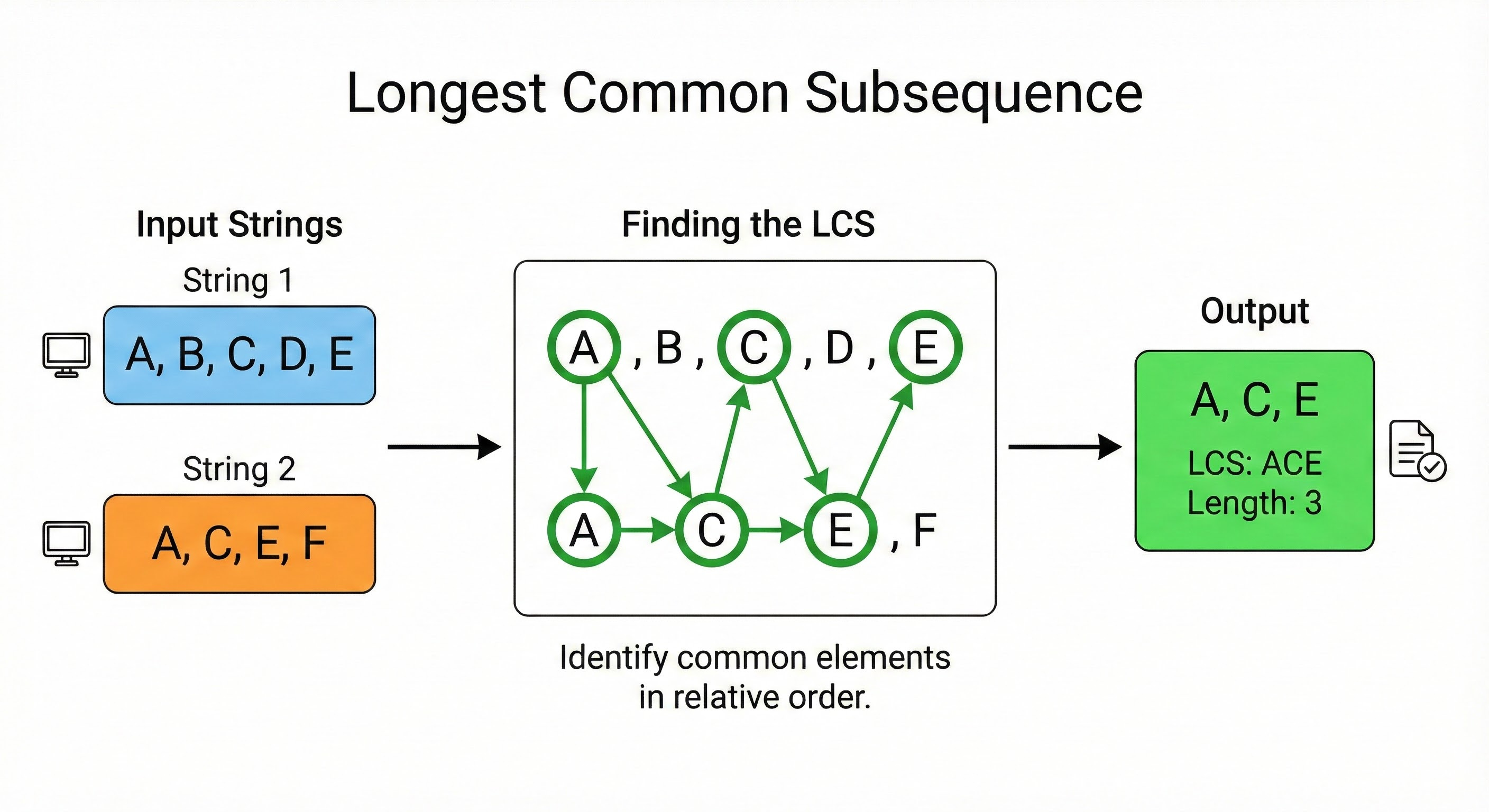
Pattern 5: Longest Common Subsequence (LCS)

This pattern deals with strings or sequences.

The Logic: You are given two strings. You want to find the length of the longest subsequence that appears in both. A subsequence is not a substring; it does not need to be consecutive, but the order must remain the same.

The State Transition: We use a 2D grid where one string is the rows and the other is the columns. We compare the character at row i with the character at column j.

Case 1: The characters match. If text1[i] == text2[j], we have found a match. We take the result from the previous diagonal (i-1, j-1) and add 1. dp[i][j] = 1 + dp[i-1][j-1]

Case 2: The characters do not match. If they are different, we cannot add to the sequence length. We must carry forward the best result we found so far.

We look at the value from the top (i-1, j) and the value from the left (i, j-1). We take the maximum of the two. dp[i][j] = max(dp[i-1][j], dp[i][j-1])

Walkthrough

1. Create a grid of size (len1 + 1) x (len2 + 1).

2. Fill the first row and column with zeros.

3. Loop through both strings.

4. If characters match, look diagonal and add 1.

5. If they differ, look top and left and take max.

Pattern 6: Palindromic Intervals

This pattern is useful for problems involving palindromes (sequences that read the same forwards and backwards).

The Logic: You define the state by two pointers, i (start) and j (end). You are looking at the substring from index i to j.

The State Transition: To determine if the string from i to j is a palindrome, you check the outer boundaries. If s[i] == s[j], then the boundaries match. Now, the condition depends on the inner substring (i+1, j-1).

If the inner substring is a palindrome AND the outer characters match, then the whole thing is a palindrome.

How to Iterate: Unlike other patterns where you iterate from 0 to N, this pattern often requires you to iterate based on the length of the substring. You solve for length 1, then length 2, then length 3, and so on.

Optimizing Space

As a senior engineer, simply solving the problem is not enough. You must optimize resources.

In many DP patterns (like the 1D Linear Scan or the Grid Traveler), you will notice that to calculate the current value, you only need the previous row or the previous value.

You do not need the entire matrix in memory.

For the 1D pattern, you only need two variables to hold prev1 and prev2. For the Grid pattern, you only need one previous row array.

This technique is called Space Optimization. It reduces the space complexity from O(N^2) or O(N) down to O(N) or O(1). Always look for this opportunity once you have a working solution.

Conclusion

Dynamic Programming is not magic. It is a systematic way of trying all possibilities but doing it efficiently. It stops you from doing the same work twice.

Here are the key takeaways to remember:

• Identify the Subproblem: Can the problem be broken down into smaller versions of itself?

• Find the Recurrence: How does the current state relate to the previous states? Write down the equation.

• Choose Your Method: Use Memoization (Top-Down) if you prefer recursion, or Tabulation (Bottom-Up) if you prefer loops.

• Initialize Base Cases: What is the answer for 0 items, 0 capacity, or an empty string?

• Optimize Space: If you only look back one step, you don’t need to store the whole history.

When you practice these patterns, do not just memorize the code.

Memorize the structure of the decision.

Understand why you look left or why you look up. Once you grasp the logic, you can adapt it to any new problem you face in an interview.