Big O Notation Explained: The Manual for Coding Interviews

Master Big O Notation and ace your coding interview. Learn to calculate Time and Space Complexity, understand the critical difference between O(n) and O(n^2 ), and write algorithms that scale.

Code often behaves differently in testing than it does in production.

A function might run instantly with fifty items but cause a system crash when processing fifty thousand.

The logic remains identical. The code works, yet the system fails.

This distinction separates basic coding from professional engineering. Solutions must survive the pressure of real-world data.

Efficiency cannot depend on guesswork. It requires a precise method to calculate how a system handles increased workloads.

This standard of measurement is called Big O Notation.

This guide explores Big O Complexity in detail. It focuses strictly on code, memory, and processor operations. The goal is to establish a clear understanding of how algorithms perform as input sizes increase.

What is Big O Notation?

Big O notation is a metric. It describes the relationship between the size of the input and the amount of resources required to process it.

In computer science, we use the variable n to represent the input size.

• If you are looping through an array of 10 numbers, n is 10.

• If you are searching through a database of 1,000,000 users, n is 1,000,000.

Big O answers a specific question: How does the workload change as n changes?

It is critical to understand that Big O does not measure speed in seconds. Measuring speed in seconds is unreliable.

A supercomputer will run a slow algorithm faster than an old laptop will run a fast algorithm.

Furthermore, background processes on your operating system can skew timing results.

Instead of seconds, we measure operations.

An operation is a basic step the computer performs, such as:

• Assigning a value to a variable.

• Comparing two numbers (x > y).

• Accessing an index in an array.

Big O describes the rate of growth.

If we double the input data, does the number of operations stay the same? Does it double? Does it quadruple?

The Worst-Case Scenario

When we analyze an algorithm, we usually look at three scenarios: Best Case, Average Case, and Worst Case.

Imagine you are iterating through a list to find a specific ID.

• Best Case: The ID is the very first item. The loop runs once.

• Worst Case: The ID is the very last item, or it does not exist at all. The loop runs n times.

In software engineering, we care almost exclusively about the Worst Case.

We are building reliability. We need to guarantee that the system will not crash even under the heaviest possible load.

If we optimize for the best case, we leave our system vulnerable.

Big O notation (specifically the “O”) formally represents this upper bound.

How to Calculate Big O

To determine the complexity of a function, you might think you need to count every single line of code.

Fortunately, that is not necessary.

We use a set of simplifying rules to determine the “Order” (that is what the O stands for).

Rule 1: Drop the Constants

Imagine a function that loops through a list of items to print them, and then loops through them again to count them.

If the list has n items, the first loop runs n times. The second loop runs n times. Mathematically, this is n + n = 2n.

In Big O analysis, we drop the constants. We do not call this O(2n). We call it O(n).

Why?

Because we are looking for the trajectory of growth, not the exact number of CPU cycles.

As n becomes massive (think billions), the difference between n and 2n is insignificant compared to the difference between n and n^2. The shape of the line on a graph is the same: it is linear.

Rule 2: Drop Non-Dominant Terms

Now imagine a function that has a nested loop (which is expensive) followed by a simple single loop.

Mathematically, the number of operations might be n^2 + n.

Here, n^2 is the dominant term.

• If n = 100, then n^2 = 10,000. The extra 100 operations from the single loop are a rounding error.

• If n = 1,000, then n^2 = 1,000,000. The extra 1,000 operations are negligible.

Because the n^2 term drives the performance cost, we ignore the smaller terms. We simplify O(n^2 + n) to just O(n^2).

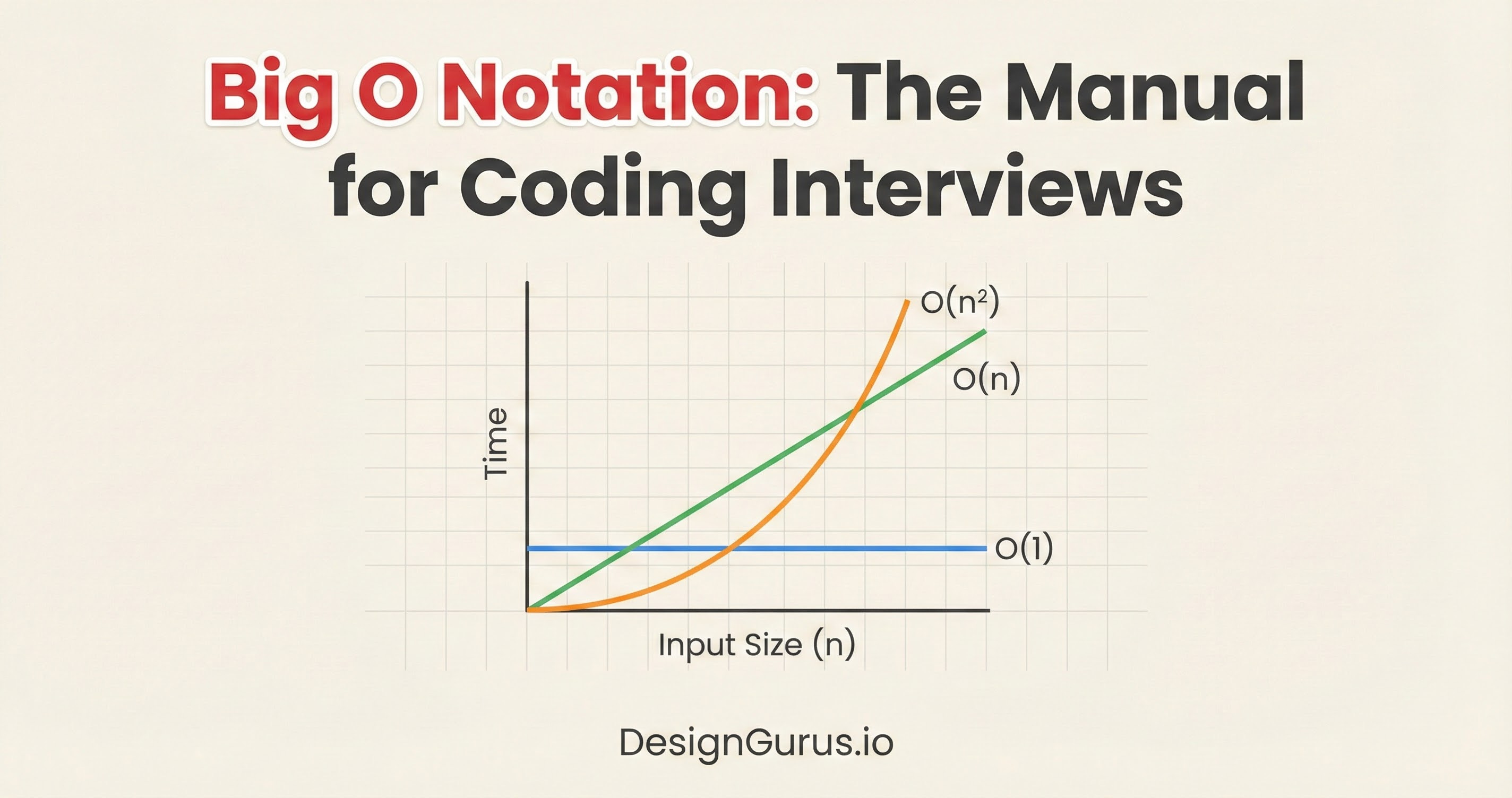
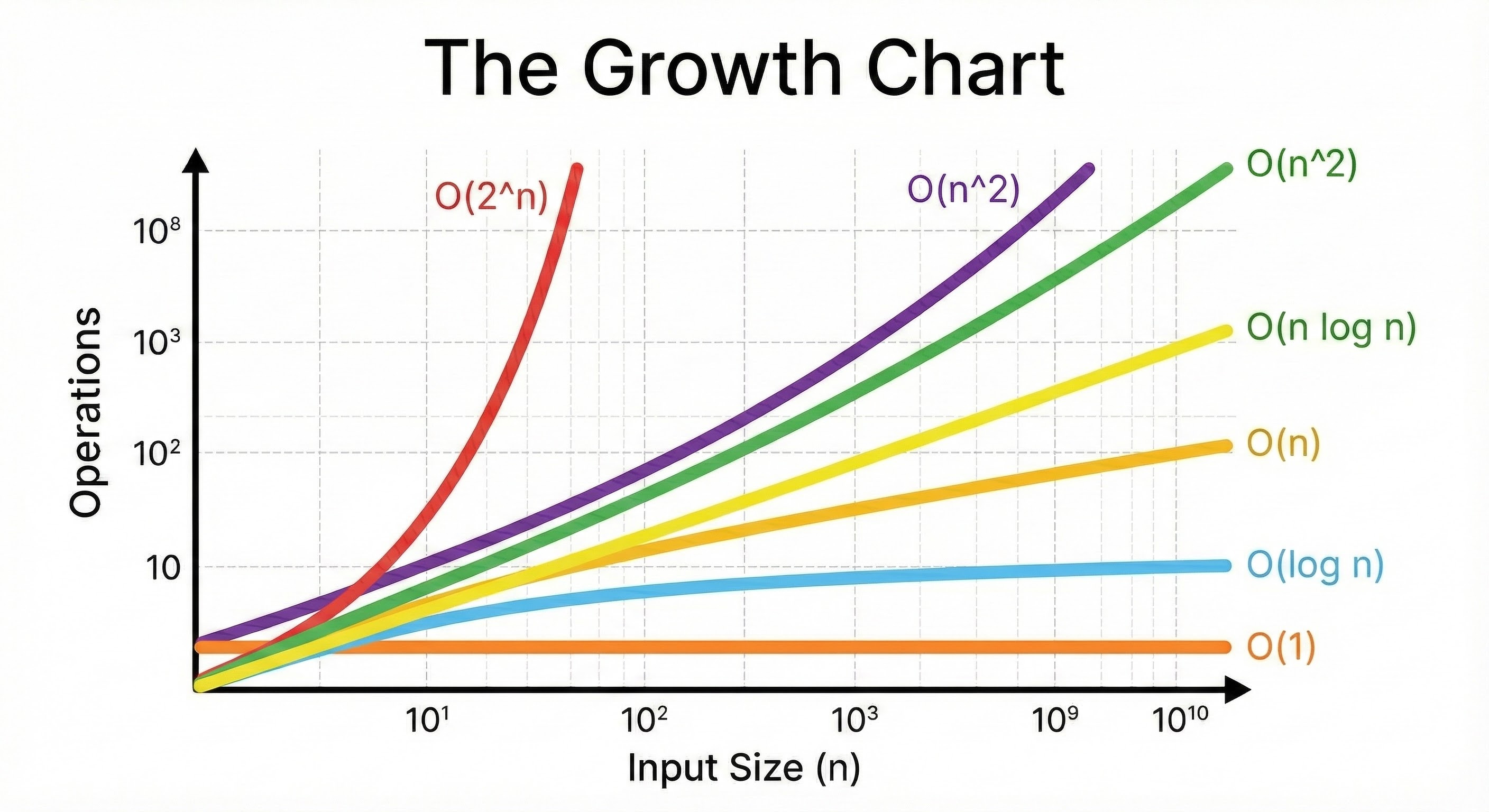
Common Time Complexities

Let’s examine the specific complexity classes you will encounter.

We will order them from the most efficient (fastest) to the least efficient (slowest).

1. O(1) : Constant Time

This is the gold standard of algorithmic efficiency. O(1) means that the execution time remains constant, regardless of the input size.

Whether your application has ten users or ten million users, this operation takes the exact same amount of time.

Code Example:

Python

def get_first_item(items):
    return items[0]

In this code, we are accessing the first element of an array.

The computer knows exactly where the array starts in memory. It goes directly to that address and reads the value. It does not scan the array. It performs one step.

Hash Maps (or Dictionaries) also provide O(1) time for lookups on average. This is why senior engineers use Hash Maps so frequently; they eliminate the need to search through data linearly.

2. O(log n) : Logarithmic Time

This is highly efficient and is the target for searching large datasets.

O(log n) means that the number of operations grows very slowly as the input grows.

This complexity usually appears in algorithms that divide the problem in half at every step.

“Log” refers to the logarithm, typically base 2 in computer science. It asks the question: “How many times must I cut n in half to get down to 1?”

• If n = 8, we cut it to 4, then 2, then 1. That is 3 steps.

• If n = 16, we cut it to 8, 4, 2, 1. That is 4 steps.

• If n = 1,000,000, it takes only roughly 20 steps.

Binary Search Example

Imagine a sorted list of numbers. You want to find the number 50. Instead of checking every number, you check the middle number.

• If the middle is 25, you know 50 is larger. You instantly ignore the entire left half of the list.

• You then check the middle of the remaining right half.

• You repeat this until you find the number.

By discarding half the data in every step, you can search massive datasets incredibly fast.

3. O(n) : Linear Time

This is the most common complexity you will write. O(n) means the runtime grows in direct proportion to the input.

If you double the input, you double the work. This typically happens when you must look at every single item in a list once.

Code Example:

Python

def print_all_items(items):
    for item in items:
        print(item)

Here, the loop runs exactly as many times as there are items.

• Input size 10 -> 10 operations.

• Input size 1,000 -> 1,000 operations.

The graph of this growth is a straight diagonal line.

O(n) is generally considered “acceptable” for most tasks, provided n does not become impossibly large.

4. O(n log n) : Linearithmic Time

This is slightly slower than linear time, but much faster than quadratic time. It is a combination of the previous two concepts: you perform a logarithmic operation n times.

This is the standard complexity for efficient Sorting Algorithms.

Mathematically, you cannot sort a generic list of numbers faster than O(n log n). Algorithms like Merge Sort, Heap Sort, and Quick Sort fall into this category.

If you use a built-in sorting function in Python (.sort()) or JavaScript (.sort()), the engine is running an O(n log n) algorithm under the hood.

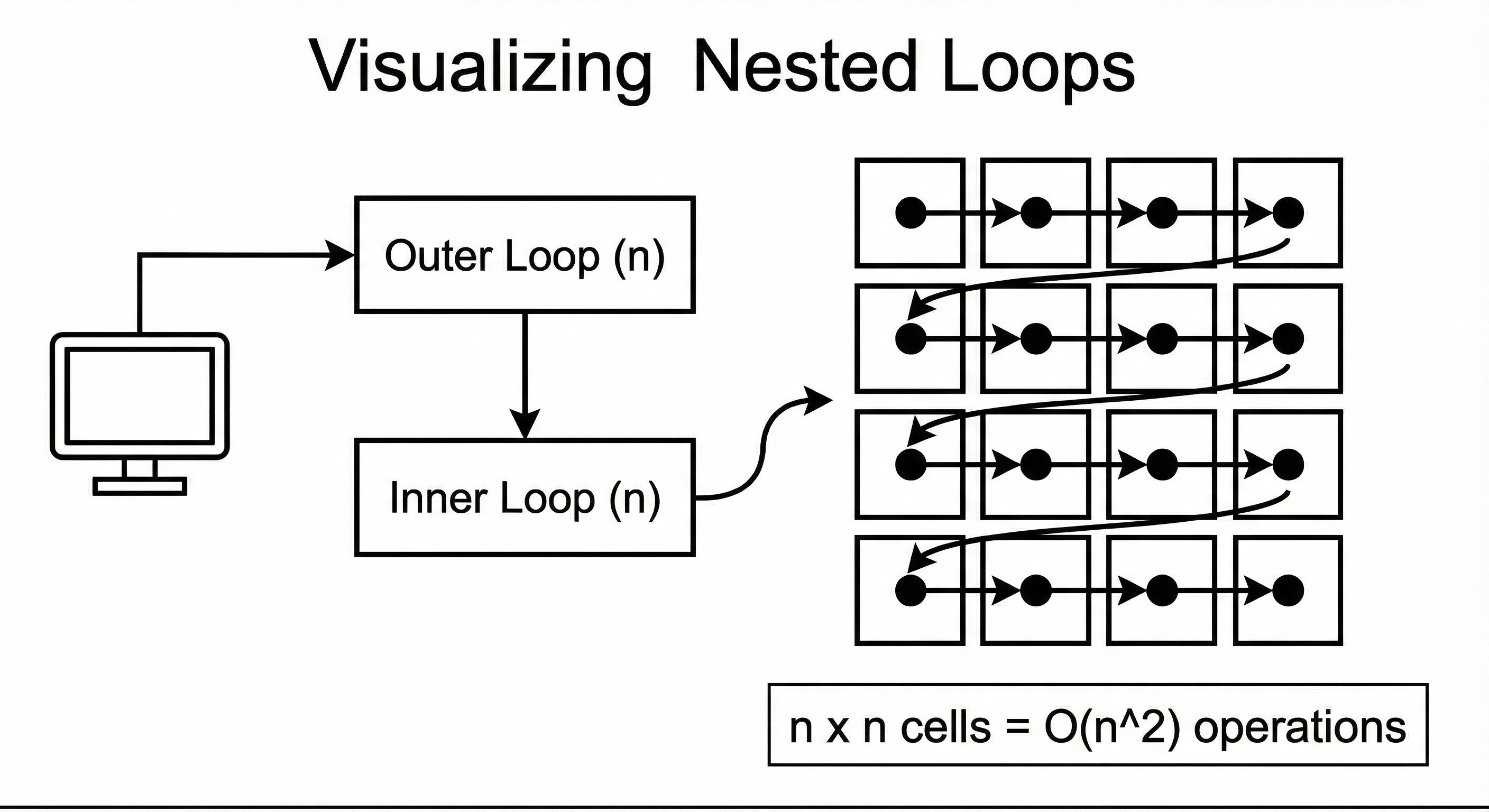
5. O(n^2) : Quadratic Time

O(n^2) means the runtime is proportional to the square of the input.

This happens when you perform a linear operation for every item in a linear dataset. The visual cue for this is Nested Loops.

Code Example:

Python

def print_pairs(items):
    for i in items:          # Outer loop
        for j in items:      # Inner loop
            print(i, j)

Let’s trace the math:

• If items has 10 elements, the outer loop runs 10 times.

• For each of those 10 times, the inner loop runs 10 times.

• Total operations: 10 x 10 = 100.

If we increase the input to 1,000:

• Total operations: 1,000 x 1,000 = 1,000,000.

Notice what happened. We increased the input by 100 times (10 to 1,000), but the workload increased by 10,000 times. This exponential curve is why servers crash.

An algorithm that is fast in testing can completely lock up a CPU when the user base grows.

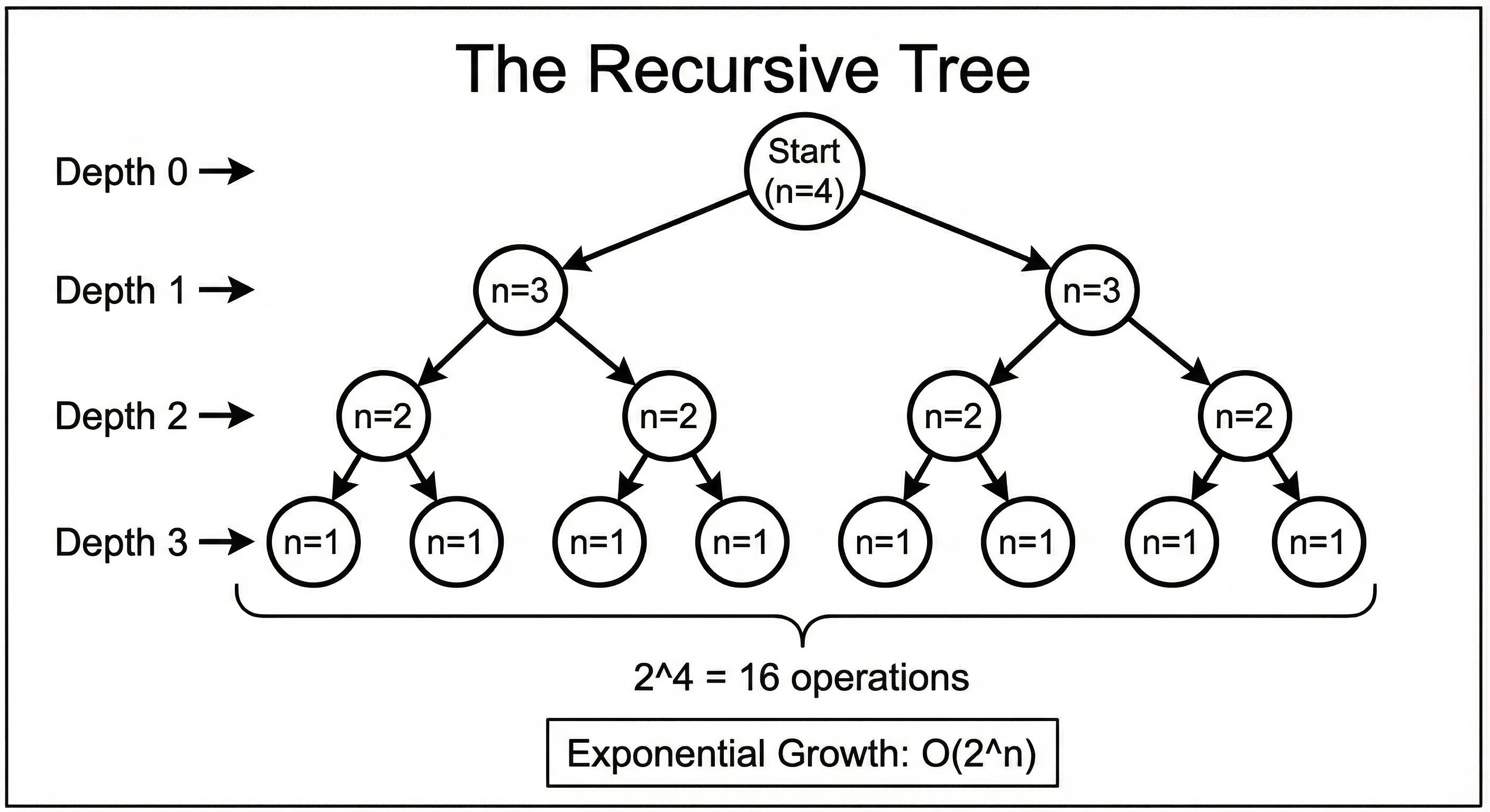
6. O(2^n) : Exponential Time

This is the “run away” complexity.

O(2^n) means that for every single element you add to the input, the required work doubles.

This is characteristic of recursive algorithms that solve a problem by branching into multiple sub-problems.

A classic example is calculating the Fibonacci sequence recursively without optimization.

• n = 10 -> ~1,000 operations.

• n = 20 -> ~1,000,000 operations.

• n = 30 -> ~1,000,000,000 operations.

By the time n reaches 40 or 50, the program could take years to finish. You should generally avoid this complexity at all costs.

Space Complexity: Memory Matters

So far, we have discussed Time Complexity (CPU operations). However, we must also consider Space Complexity (RAM usage).

Just like time, we measure space by how it grows relative to the input.

O(1) Space

The algorithm uses a fixed amount of memory. It creates a few variables (counters, sums, temporary holders), but it does not allocate large data structures.

• Example: looping through a list and summing the numbers.

O(n) Space

The algorithm allocates memory proportional to the input size.

• Example: Copying a list into a new list. If the original list is 1GB, you need another 1GB of RAM.

The Hidden Cost of Recursion

One specific area that trips up junior developers is Stack Space.

When a function calls itself (recursion), the computer must “remember” the previous function call so it can return to it later. It stores this on the Call Stack.

If you have a recursive function that calls itself n times deeply, you are using O(n) space in memory, even if you are not creating new arrays.

If n is too large, you will run out of stack memory and crash the program (a Stack Overflow).

A Senior Engineer’s Mental Checklist

When you are writing code or performing a code review, you do not need to write out mathematical proofs. You can use a mental heuristic to quickly estimate Big O.

1. Identify the Loops: Look at the for and while loops.

2. Check for Nesting: Is there a loop inside another loop?

   • If yes, are they iterating over the same collection? That is likely O(n^2).

   • If no, and they are side-by-side, that is likely O(n).

3. Check Function Calls: Does the loop call a helper function?

   • If the loop runs n times, and the helper function inside it also takes O(n) time, the total is O(n^2).

4. Look for Division: Is the input size being cut in half repeatedly? That is O(log n).

5. Check Memory: Are you creating a new list for every item you process? That is O(n) space.

Conclusion

Mastering Big O complexity is a major milestone in your development career. It shifts your perspective from “getting code to work” to “engineering systems that last.”

It enables you to look at a solution and predict its failure points before they happen. It allows you to argue for code refactoring with data rather than opinions.

Here are the key takeaways to remember:

• Big O measures growth. It tells us how the workload increases as the data increases.

• Worst Case is key. We plan for the heaviest load to ensure reliability.

• O(1) and O(log n) are excellent. These are the goals for scalable systems.

• O(n) is standard. Linear time is acceptable for simple data processing.

• O(n^2) is dangerous. Nested loops should be treated with caution and optimized if the dataset is large.

• Space is a resource. Always consider how much RAM your solution requires, especially with recursion or large array copies.

The next time you write a function, pause for a moment.

Ask yourself: “If I pass a million items into this, what happens?” The answer to that question is the essence of Big O.